Capture the Dominant Spatial Pattern with Two-Dimensional Locations

Objective

Represent how to use SpatPCA for two-dimensional data for capturing the most dominant spatial pattern

Basic settings

Used packages

library(SpatPCA)
library(ggplot2)
library(dplyr)
library(tidyr)
library(gifski)
library(fields)
library(scico)

base_theme <- theme_minimal(base_size = 10, base_family = "Times") +
  theme(legend.position = "bottom")
fill_bar <- guides(fill = guide_colourbar(
  barwidth = 10,
  barheight = 0.5,
  label.position = "bottom"
))
coltab <- scico(128, palette = "vik")
color_scale_limit <- c(-.8, .8)

True spatial pattern (eigenfunction)

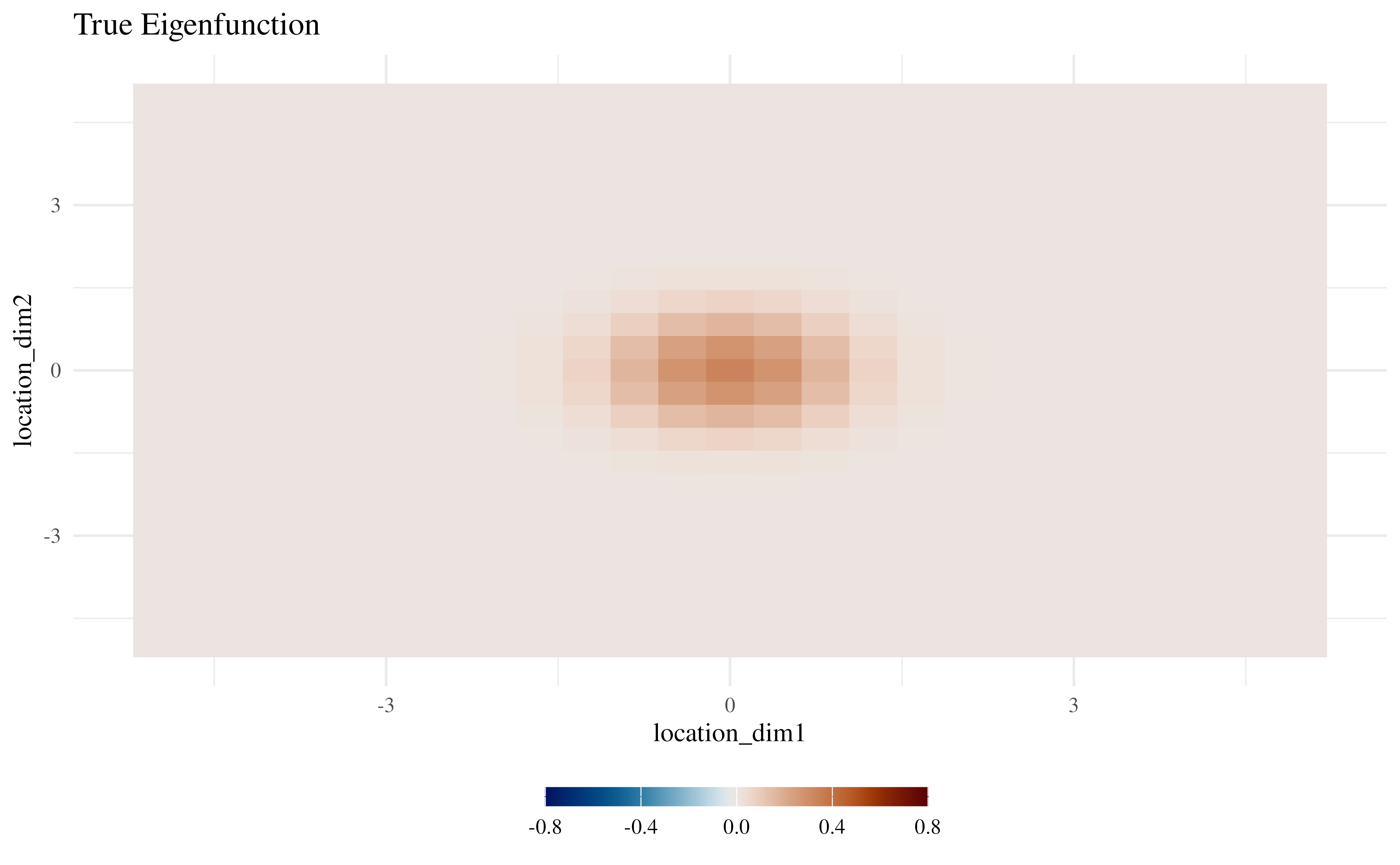
The underlying spatial pattern below indicates realizations will vary dramatically at the center and be almost unchanged at the both ends of the curve.

set.seed(1024)
p <- 25
n <- 8
location <-
  matrix(rep(seq(-5, 5, length = p), 2), nrow = p, ncol = 2)
expanded_location <- expand.grid(location[, 1], location[, 2])
unnormalized_eigen_fn <-
  as.vector(exp(-location[, 1]^2) %*% t(exp(-location[, 2]^2)))
true_eigen_fn <-
  unnormalized_eigen_fn / norm(t(unnormalized_eigen_fn), "F")

data.frame(
  location_dim1 = expanded_location[, 1],
  location_dim2 = expanded_location[, 2],
  eigenfunction = true_eigen_fn
) %>%
  ggplot(aes(location_dim1, location_dim2)) +
  geom_tile(aes(fill = eigenfunction)) +
  scale_fill_gradientn(colours = coltab, limits = color_scale_limit) +
  base_theme +
  labs(title = "True Eigenfunction", fill = "") +
  fill_bar

Experiment

Generate 2-D realizations

We want to generate 100 random sample based on
- The spatial signal for the true spatial pattern is distributed normally with $\sigma=20$
- The noise follows the standard normal distribution.

realizations <- rnorm(n = n, sd = 3) %*% t(true_eigen_fn) + matrix(rnorm(n = n * p^2), n, p^2)

Animate realizations

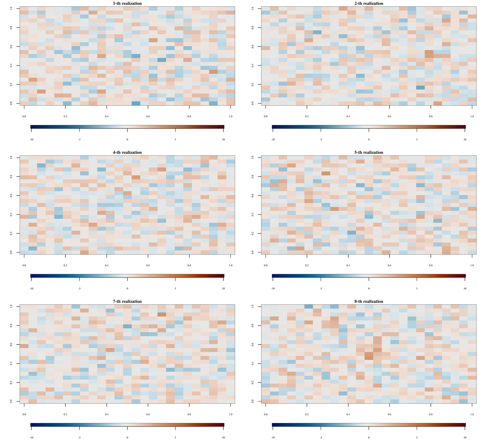
We can see simulated central realizations change in a wide range more frequently than the others.

original_par <- par()
for (i in 1:n) {
  par(mar = c(3, 3, 1, 1), family = "Times")
  image.plot(
    matrix(realizations[i, ], p, p),
    main = paste0(i, "-th realization"),
    zlim = c(-10, 10),
    col = coltab,
    horizontal = TRUE,
    cex.main = 0.8,
    cex.axis = 0.5,
    axis.args = list(cex.axis = 0.5),
    legend.width = 0.5
  )
}

par(original_par)
#> Warning in par(original_par): graphical parameter "cin" cannot be set
#> Warning in par(original_par): graphical parameter "cra" cannot be set
#> Warning in par(original_par): graphical parameter "csi" cannot be set
#> Warning in par(original_par): graphical parameter "cxy" cannot be set
#> Warning in par(original_par): graphical parameter "din" cannot be set
#> Warning in par(original_par): graphical parameter "page" cannot be set

Apply `SpatPCA::spatpca`

We add a candidate set of tau2 to see how SpatPCA obtain a localized smooth pattern.

tau2 <- c(0, exp(seq(log(10), log(400), length = 10)))
cv <- spatpca(x = expanded_location, Y = realizations, tau2 = tau2)
eigen_est <- cv$eigenfn

Compare SpatPCA with PCA

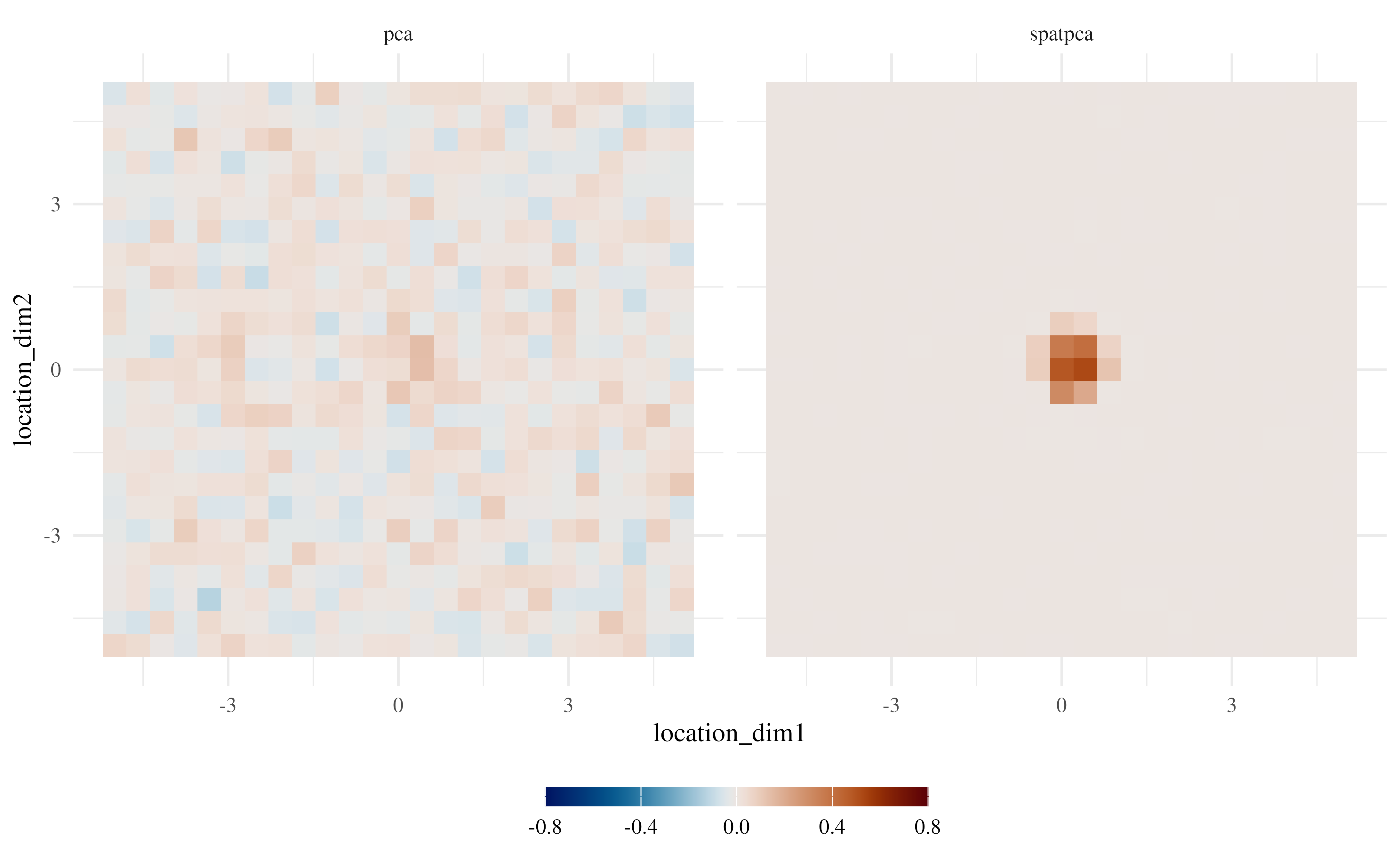
The following figure shows that SpatPCA can find sparser pattern than PCA, which is close to the true pattern.

data.frame(
  location_dim1 = expanded_location[, 1],
  location_dim2 = expanded_location[, 2],
  spatpca = eigen_est[, 1],
  pca = svd(realizations)$v[, 1]
) %>%
  gather(estimate, eigenfunction, -c(location_dim1, location_dim2)) %>%
  ggplot(aes(location_dim1, location_dim2)) +
  geom_tile(aes(fill = eigenfunction)) +
  scale_fill_gradientn(colours = coltab, limits = color_scale_limit) +
  base_theme +
  facet_wrap(. ~ estimate) +
  labs(fill = "") +
  fill_bar

Wen-Ting Wang