Capture the Dominant Spatial Pattern with One-Dimensional Locations

Wen-Ting Wang

Objective

We have two objectives 1. Demonstrate how SpatPCA captures the most dominant spatial pattern of variation based on different signal-to-noise ratios. 2. Represent how to use SpatPCA for one-dimensional data

Basic settings

Used packages

library(SpatPCA)
library(ggplot2)
library(dplyr)
library(tidyr)
library(gifski)
base_theme <- theme_classic(base_size = 18, base_family = "Times")

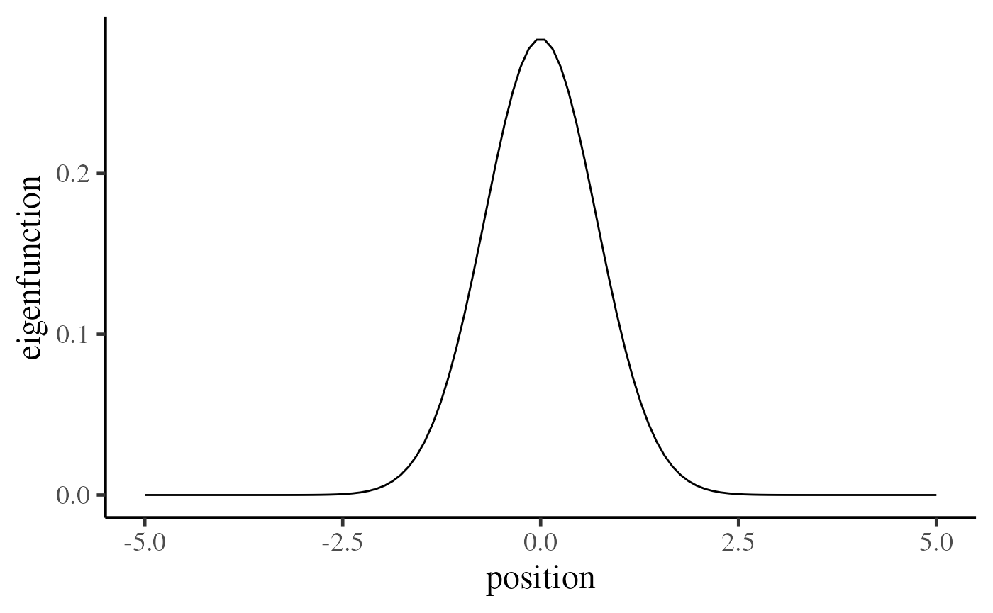
True spatial pattern (eigenfunction)

The underlying spatial pattern below indicates realizations will vary dramatically at the center and be almost unchanged at the both ends of the curve.

set.seed(1024)
position <- matrix(seq(-5, 5, length = 100))
true_eigen_fn <- exp(-position^2) / norm(exp(-position^2), "F")

data.frame(
  position = position,
  eigenfunction = true_eigen_fn
) %>%
  ggplot(aes(position, eigenfunction)) +
  geom_line() +
  base_theme

Case I: Higher signal of the true eigenfunction

Generate realizations

We want to generate 100 random sample based on - The spatial signal for the true spatial pattern is distributed normally with $\sigma=20$ - The noise follows the standard normal distribution.

realizations <- rnorm(n = 100, sd = 20) %*% t(true_eigen_fn) + matrix(rnorm(n = 100 * 100), 100, 100)

Animate realizations

We can see simulated central realizations change in a wide range more frequently than the others.

for (i in 1:100) {
  plot(x = position, y = realizations[i, ], ylim = c(-10, 10), ylab = "realization")
}

Apply SpatPCA::spatpca

cv <- spatpca(x = position, Y = realizations)
eigen_est <- cv$eigenfn

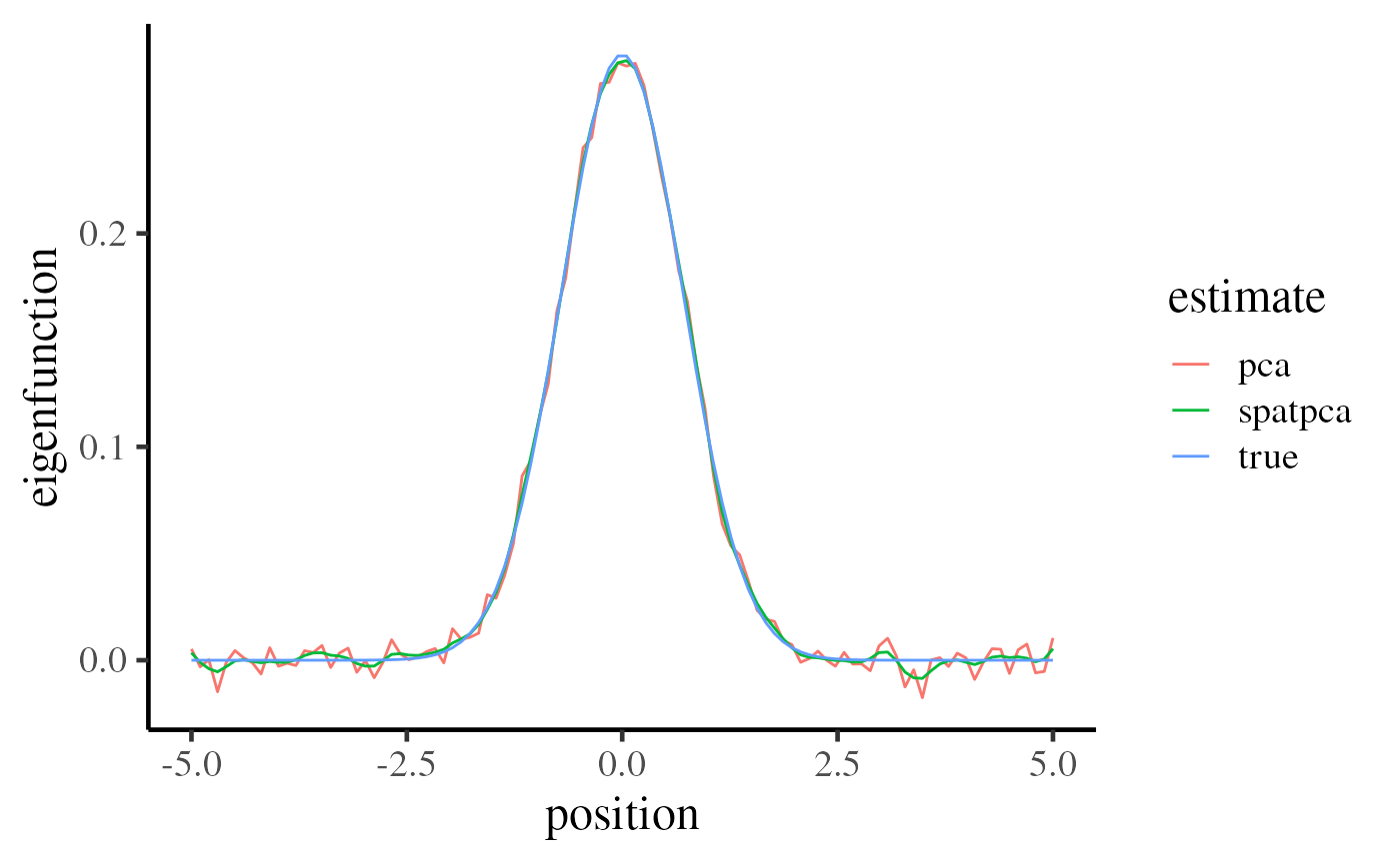
Compare SpatPCA with PCA

There are two comparison remarks 1. Two estimates are similar to the true eigenfunctions 2. SpatPCA can perform better at the both ends.

data.frame(
  position = position,
  true = true_eigen_fn,
  spatpca = eigen_est[, 1],
  pca = svd(realizations)$v[, 1]
) %>%
  gather(estimate, eigenfunction, -position) %>%
  ggplot(aes(x = position, y = eigenfunction, color = estimate)) +
  geom_line() +
  base_theme

Case II: Lower signal of the true eigenfunction

Generate realizations with $\sigma=3$

realizations <- rnorm(n = 100, sd = 3) %*% t(true_eigen_fn) + matrix(rnorm(n = 100 * 100), 100, 100)

Animate realizations

It is hard to see a crystal clear spatial pattern via the simulated sample shown below.

for (i in 1:100) {
  plot(x = position, y = realizations[i, ], ylim = c(-10, 10), ylab = "realization")
}

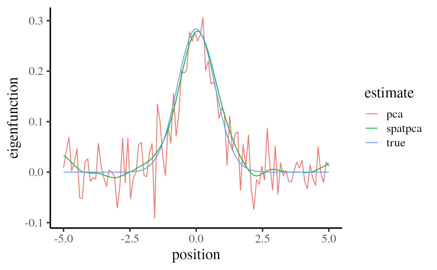
Compare resultant patterns

The following panel indicates that SpatPCA outperforms to PCA visually when the signal-to-noise ratio is quite lower.

cv <- spatpca(x = position, Y = realizations)
eigen_est <- cv$eigenfn

data.frame(
  position = position,
  true = true_eigen_fn,
  spatpca = eigen_est[, 1],
  pca = svd(realizations)$v[, 1]
) %>%
  gather(estimate, eigenfunction, -position) %>%
  ggplot(aes(x = position, y = eigenfunction, color = estimate)) +
  geom_line() +
  base_theme