This function performs resolution adaptive fixed rank kriging based on spatial data observed at one or multiple time points via the following spatial random-effects model: $$z[t]=\mu + G \cdot w[t]+\eta[t]+e[t], w[t] \sim N(0,M), e[t] \sim N(0, s \cdot D); t=1,...,T,$$ where \(z[t]\) is an n-vector of (partially) observed data at n locations, \(\mu\) is an n-vector of deterministic mean values, \(D\) is a given n by n matrix, \(G\) is a given n by K matrix, \(\eta[t]\) is an n-vector of random variables corresponding to a spatial stationary process, and \(w[t]\) is a K-vector of unobservable random weights. Parameters are estimated by maximum likelihood in a closed-form expression. The matrix \(G\) corresponding to basis functions is given by an ordered class of thin-plate spline functions, with the number of basis functions selected by Akaike's information criterion.
Arguments
- data
n by T data matrix (NA allowed) with \(z[t]\) as the t-th column.
- loc
n by d matrix of coordinates corresponding to n locations.
- mu
n-vector or scalar for \(\mu\); Default is 0.
- D
n by n matrix (preferably sparse) for the covariance matrix of the measurement errors up to a constant scale. Default is an identity matrix.
- G
n by K matrix of basis function values with each column being a basis function taken values at
loc. Default is NULL, which is automatic determined.- finescale
logical; if
TRUEthen a (approximate) stationary finer scale process \(\eta[t]\) will be included based onLatticeKrigpacakge. In such a case, only the diagonals of \(D\) would be taken into account. Default isFALSE.- maxit
maximum number of iterations. Default is 50.
- tolerance
precision tolerance for convergence check. Default is 0.1^6.
- maxK
maximum number of basis functions considered. Default is \(10 \cdot \sqrt{n}\) for n>100 or n for n<=100.
- Kseq
user-specified vector of numbers of basis functions considered. Default is
NULL, which is determined frommaxK.- method
"fast" or " EM"; if "fast" then the missing data are filled in using k-nearest-neighbor imputation; if "EM" then the missing data are taken care by the EM algorithm. Default is "fast".
- n.neighbor
number of neighbors to be used in the "fast" imputation method. Default is 3.
- maxknot
maximum number of knots to be used in generating basis functions. Default is 5000.
Value
an object of class FRK is returned, which is a list of the following components:
- M
ML estimate of \(M\).
- s
estimate for the scale parameter of measurement errors.
- negloglik
negative log-likelihood.
- w
K by T matrix with \(w[t]\) as the t-th column.
- V
K by K matrix of the prediction error covariance matrix of \(w[t]\).
- G
user specified basis function matrix or an automatically generated
mrtsobject.- LKobj
a list from calling
LKrig.MLEinLatticeKrigpackage ifuseLK=TRUE; otherwiseNULL. See that package for details.
Details
The function computes the ML estimate of M using the closed-form expression in Tzeng and Huang (2018).
If the user would like to specify
a D other than an identity matrix for a large n, it is better to provided via spam function
in spam package.
References
Tzeng, S., & Huang, H.-C. (2018). Resolution Adaptive Fixed Rank Kriging, Technometrics, https://doi.org/10.1080/00401706.2017.1345701.
Nychka D, Hammerling D, Sain S, Lenssen N (2016). “LatticeKrig: Multiresolution Kriging Based on Markov Random Fields.” doi:10.5065/D6HD7T1R https://doi.org/10.5065/D6HD7T1R, R package version 8.4, https://github.com/NCAR/LatticeKrig.
See also
Examples
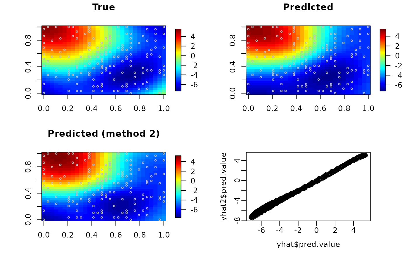
#### generating data from two eigenfunctions
originalPar <- par(no.readonly = TRUE)
set.seed(0)
n <- 150
s <- 5
grid1 <- grid2 <- seq(0, 1, l = 30)
grids <- expand.grid(grid1, grid2)
fn <- matrix(0, 900, 2)
fn[, 1] <- cos(sqrt((grids[, 1] - 0)^2 + (grids[, 2] - 1)^2) * pi)
fn[, 2] <- cos(sqrt((grids[, 1] - 0.75)^2 + (grids[, 2] - 0.25)^2) * 2 * pi)

#### single realization simulation example
w <- c(rnorm(1, sd = 5), rnorm(1, sd = 3))
y <- fn %*% w
obs <- sample(900, n)
z <- y[obs] + rnorm(n) * sqrt(s)
X <- grids[obs, ]

#### method1: automatic selection and prediction
one.imat <- autoFRK(data = z, loc = X, maxK = 15)
yhat <- predict(one.imat, newloc = grids)

#### method2: user-specified basis functions
G <- mrts(X, 15)
Gpred <- predict(G, newx = grids)
one.usr <- autoFRK(data = z, loc = X, G = G)
yhat2 <- predict(one.usr, newloc = grids, basis = Gpred)

require(fields)
#> Loading required package: fields
#> Loading required package: viridisLite
#>
#> Try help(fields) to get started.
par(mfrow = c(2, 2))
image.plot(matrix(y, 30, 30), main = "True")
points(X, cex = 0.5, col = "grey")
image.plot(matrix(yhat$pred.value, 30, 30), main = "Predicted")
points(X, cex = 0.5, col = "grey")
image.plot(matrix(yhat2$pred.value, 30, 30), main = "Predicted (method 2)")
points(X, cex = 0.5, col = "grey")
plot(yhat$pred.value, yhat2$pred.value, mgp = c(2, 0.5, 0))

par(originalPar)
#### end of single realization simulation example

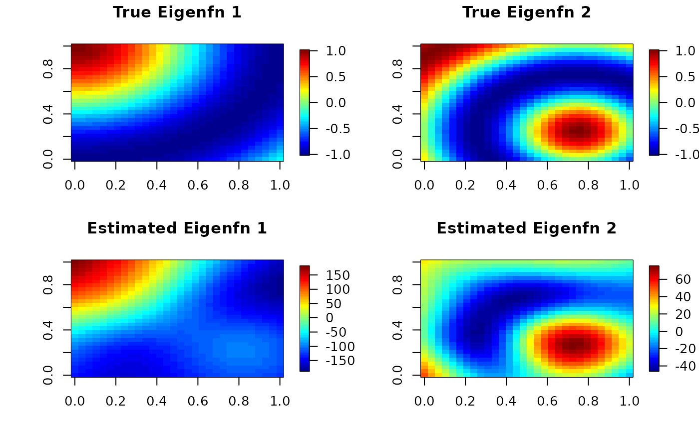
#### independent multi-realization simulation example
set.seed(0)
wt <- matrix(0, 2, 20)
for (tt in 1:20) wt[, tt] <- c(rnorm(1, sd = 5), rnorm(1, sd = 3))
yt <- fn %*% wt
obs <- sample(900, n)
zt <- yt[obs, ] + matrix(rnorm(n * 20), n, 20) * sqrt(s)
X <- grids[obs, ]
multi.imat <- autoFRK(data = zt, loc = X, maxK = 15)
Gpred <- predict(multi.imat$G, newx = grids)

G <- multi.imat$G
Mhat <- multi.imat$M
dec <- eigen(G %*% Mhat %*% t(G))
fhat <- Gpred %*% Mhat %*% t(G) %*% dec$vector[, 1:2]
par(mfrow = c(2, 2))
image.plot(matrix(fn[, 1], 30, 30), main = "True Eigenfn 1")
image.plot(matrix(fn[, 2], 30, 30), main = "True Eigenfn 2")
image.plot(matrix(fhat[, 1], 30, 30), main = "Estimated Eigenfn 1")
image.plot(matrix(fhat[, 2], 30, 30), main = "Estimated Eigenfn 2")

par(originalPar)
#### end of independent multi-realization simulation example