Produce spatial coupled patterns at the designated locations according to the specified tuning parameters or the tuning parameters selected by M-fold cross-validation.
Arguments
- x1
Location matrix (\(p \times d\)) corresponding to Y1. Each row is a location. \(d=1,2\) is the dimension of locations.
- x2
Location matrix (\(q \times d\)) corresponding to Y2. Each row is a location.
- Y1
Data matrix (\(n \times p\)) of the first variable stores the values at \(p\) locations with sample size \(n\).
- Y2
Data matrix (\(n \times q\)) of the second variable stores the values at \(q\) locations with sample size \(n\).
- M
Optional number of folds; default is 5.
- K
Optional user-supplied number of coupled patterns; default is NULL. If K is NULL or is_K_selected is TRUE, K is selected automatically.
- is_K_selected
If TRUE, K is selected automatically; otherwise, is_K_selected is set to be user-supplied K. Default depends on user-supplied K.
- tau1u
Optional user-supplied numeric vector of a nonnegative smoothness parameter sequence corresponding to Y1. If NULL, 10 tau1u values in a range are used.
- tau2u
Optional user-supplied numeric vector of a nonnegative smoothness parameter sequence corresponding to Y1. If NULL, 10 tau2u values in a range are used.
- tau1v
Optional user-supplied numeric vector of a nonnegative smoothness parameter sequence corresponding to Y2. If NULL, 10 tau1v values in a range are used.
- tau2v
Optional user-supplied numeric vector of a nonnegative smoothness parameter sequence corresponding to Y2. If NULL, 10 tau2v values in a range are used.
- x1New
New location matrix corresponding to Y1. If NULL, it is x1.
- x2New
New location matrix corresponding to Y2. If NULL, it is x2.
- center
If TRUE, center the columns of Y. Default is FALSE.
- maxit
Maximum number of iterations. Default value is 100.
- thr
Threshold for convergence. Default value is \(10^{-4}\).
- are_all_tuning_parameters_selected
If TRUE, the K-fold CV performs to select 4 tuning parameters simultaneously. Default value is FALSE.
- num_cores
Number of cores used to parallel computing. Default value is NULL (See
RcppParallel::defaultNumThreads())
Value
A list of objects including
- Uestfn
Estimated patterns for Y1 at the new locations, x1New.
- Vestfn
Estimated patterns for Y2 at the new locations, x2New.
- Dest
Estimated singular values.
- crosscov
Estimated cross-covariance matrix between Y1 and Y2.
- stau1u
Selected tau1u.
- stau2u
Selected tau2u.
- stau1v
Selected tau1v.
- stau2v
Selected tau2v.
- cv1
cv scores for tau1u and tau1v when are_all_tuning_parameters_selected is FALSE.
- cv2
cv scores for tau2u and tau2v when are_all_tuning_parameters_selected is FALSE.
- cvall
cv scores for tau1u, tau2u, tau1v and tau2v when are_all_tuning_parameters_selected is TRUE.
- tau1u
Sequence of tau1u-values used in the process.
- tau2u
Sequence of tau2u-values used in the process.
- tau1v
Sequence of tau1v-values used in the process.
- tau2v
Sequence of tau2v-values used in the process.
Details
The optimization problem is $$\max_{\mathbf{U}, \mathbf{V}} \frac{1}{n}\mbox{tr}(\mathbf{U}'\mathbf{Y}'_1\mathbf{Y}_2\mathbf{V}) - \tau_{1u}\mbox{tr}(\mathbf{U}'\mathbf{\Omega}_1\mathbf{U}) - \tau_{2u}\sum_{k=1}^K\sum_{j=1}^{p} |u_{jk}|- \tau_{1v}\mbox{tr}(\mathbf{V}'\mathbf{\Omega}_2\mathbf{V})-\tau_{2v}\sum_{k=1}^K\sum_{j=1}^{q} |v_{jk}|,$$ \(\mbox{subject to $ \mathbf{U}'\mathbf{U}=\mathbf{V}'\mathbf{V}=\mathbf{I}_K$,}\) where \(\mathbf{Y}_1\) and \(\mathbf{Y}_2\) are two data matrices, \({\mathbf{\Omega}}_1\) and \({\mathbf{\Omega}}_2\) are two smoothness matrix, \(\mathbf{V}=\{v_{jk}\}\), and \(\mathbf{U}=\{u_{jk}\}\).
References
Wang, W.-T. and Huang, H.-C. (2017). Regularized principal component analysis for spatial data. Journal of Computational and Graphical Statistics 26 14-25.
Examples
originalPar <- par(no.readonly = TRUE)
# The following examples only use two threads for parallel computing.
## 1D: regular locations
p <- q <- 10
n <- 100
x1 <- matrix(seq(-7, 7, length = p), nrow = p, ncol = 1)
x2 <- matrix(seq(-7, 7, length = q), nrow = q, ncol = 1)
u <- exp(-x1^2) / norm(exp(-x1^2), "F")
v <- exp(-(x2 - 2)^2) / norm(exp(-(x2 - 2)^2), "F")
Sigma <- array(0, c(p + q, p + q))
Sigma[1:p, 1:p] <- diag(p)
Sigma[(p + 1):(p + q), (p + 1):(p + q)] <- diag(p)
Sigma[1:p, (p + 1):(p + q)] <- u %*% t(v)
Sigma[(p + 1):(p + q), 1:p] <- t(Sigma[1:p, (p + 1):(p + q)])
noise <- MASS::mvrnorm(n, mu = rep(0, p + q), Sigma = 0.001 * diag(p + q))
Y <- MASS::mvrnorm(n, mu = rep(0, p + q), Sigma = Sigma) + noise
Y1 <- Y[, 1:p]
Y2 <- Y[, -(1:p)]
cv1 <- spatmca(x1, x2, Y1, Y2, num_cores = 2)

par(mfrow = c(2, 1))
plot(x1, cv1$Uestfn[, 1], type='l', main = "1st pattern for Y1")
plot(x1, cv1$Vestfn[, 1], type='l', main = "1st pattern for Y2")

## Avoid changing the global enviroment
par(originalPar)

# \donttest{
# The following examples will be executed more than 5 secs or including other libraries.
## 1D: artificial irregular locations
rmLoc1 <- sample(1:p, 3)
rmLoc2 <- sample(1:q, 4)
x1Rm <- x1[-rmLoc1]
x2Rm <- x2[-rmLoc2]
Y1Rm <- Y1[, -rmLoc1]
Y2Rm <- Y2[, -rmLoc2]
x1New <- as.matrix(seq(-7, 7, length = 100))
x2New <- as.matrix(seq(-7, 7, length = 50))
cv2 <- spatmca(x1 = x1Rm,
               x2 = x2Rm,
               Y1 = Y1Rm,
               Y2 = Y2Rm,
               x1New = x1New,
               x2New = x2New)
par(mfrow = c(2, 1))
plot(x1New, cv2$Uestfn[,1], type='l', main = "1st pattern for Y1")
plot(x2New, cv2$Vestfn[,1], type='l', main = "1st pattern for Y2")

par(originalPar)

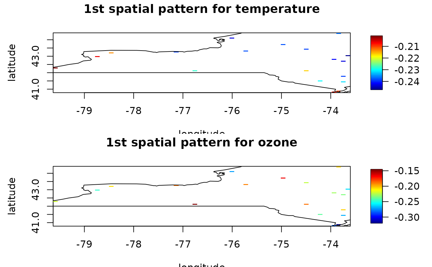
## 2D real data
##  Daily 8-hour ozone averages and maximum temperature obtained from 28 monitoring
##  sites of NewYork, USA. It is of interest to see the relationship between the ozone
##  and the temperature through the coupled patterns.

library(spTimer)
#>
#> ## spTimer version: 3.3.2
library(pracma)
#>
#> Attaching package: ‘pracma’
#> The following object is masked from ‘package:spTimer’:
#>
#>     Norm
#> The following object is masked from ‘package:SpatMCA’:
#>
#>     detrend
library(fields)
#> Loading required package: spam
#> Spam version 2.10-0 (2023-10-23) is loaded.
#> Type 'help( Spam)' or 'demo( spam)' for a short introduction
#> and overview of this package.
#> Help for individual functions is also obtained by adding the
#> suffix '.spam' to the function name, e.g. 'help( chol.spam)'.
#>
#> Attaching package: ‘spam’
#> The following objects are masked from ‘package:base’:
#>
#>     backsolve, forwardsolve
#> Loading required package: viridisLite
#>
#> Try help(fields) to get started.
library(maps)
data(NYdata)
NYsite <- unique(cbind(NYdata[, 1:3]))
date <- as.POSIXct(seq(as.Date("2006-07-01"), as.Date("2006-08-31"), by = 1))
cMAXTMP<- matrix(NYdata[,8], 62, 28)
oz <- matrix(NYdata[,7], 62, 28)
rmNa <- !colSums(is.na(oz))
temp <- detrend(matrix(cMAXTMP[, rmNa], nrow = nrow(cMAXTMP)), "linear")
ozone <- detrend(matrix(oz[, rmNa], nrow = nrow(oz)), "linear")
x1 <- NYsite[rmNa, 2:3]
cv <- spatmca(x1, x1, temp, ozone)
par(mfrow = c(2, 1))
quilt.plot(x1, cv$Uestfn[, 1],
           xlab = "longitude",
           ylab = "latitude",
           main = "1st spatial pattern for temperature")
map(database = "state", regions = "new york", add = TRUE)
quilt.plot(x1, cv$Vestfn[, 1],
           xlab = "longitude",
           ylab = "latitude",
           main = "1st spatial pattern for ozone")
map(database = "state", regions = "new york", add = TRUE)

par(originalPar)

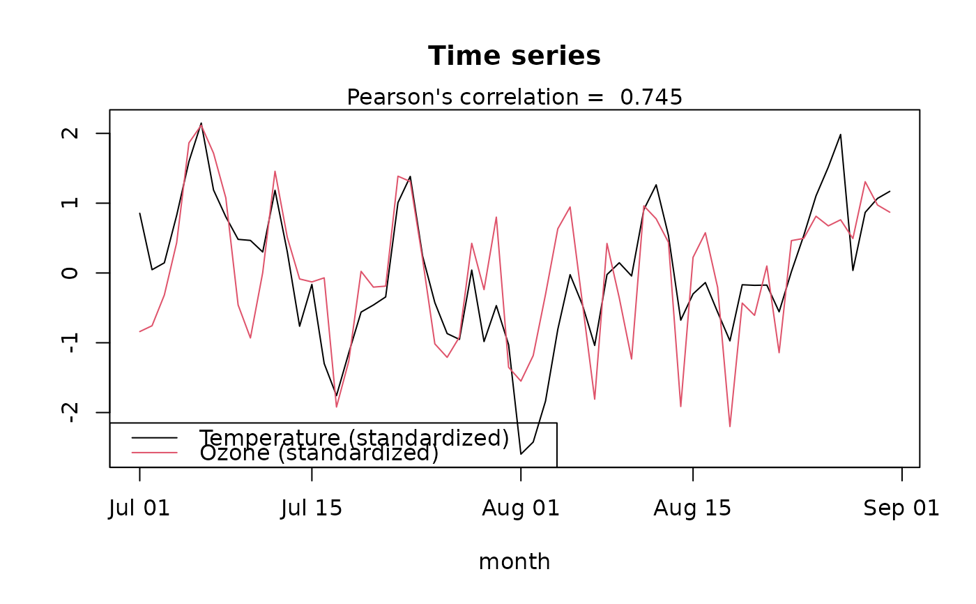
### Time series for the coupled patterns
tstemp <- temp %*% cv$Uestfn[,1]
tsozone <- ozone %*% cv$Vestfn[,1]
corr <- cor(tstemp, tsozone)
plot(date, tstemp / sd(tstemp), type='l', main = "Time series", ylab = "", xlab = "month")
lines(date, tsozone/sd(tsozone),col=2)
legend("bottomleft", c("Temperature (standardized)", "Ozone (standardized)"), col = 1:2, lty = 1:1)
mtext(paste("Pearson's correlation = ", round(corr, 3)), 3)


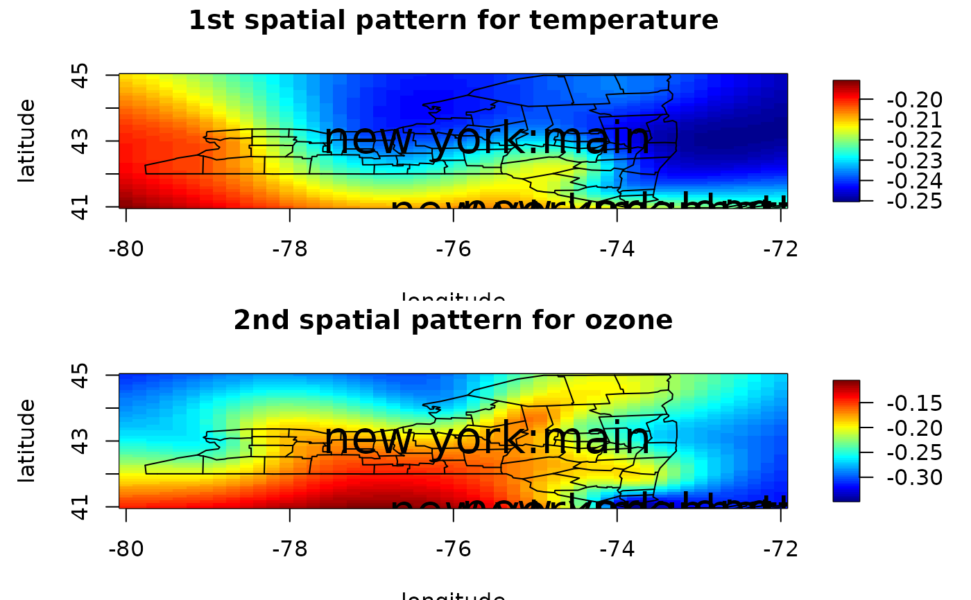
newP <- 50
xLon <- seq(-80, -72, length = newP)
xLat <- seq(41, 45, length = newP)
xxNew <- as.matrix(expand.grid(x = xLon, y = xLat))
cvNew <- spatmca(x1 = x1,
                 x2 = x1,
                 Y1 = temp,
                 Y2 = ozone,
                 K = cv$Khat,
                 tau1u = cv$stau1u,
                 tau1v = cv$stau1v,
                 tau2u = cv$stau2u,
                 tau2v = cv$stau2v,
                 x1New = xxNew,
                 x2New = xxNew)
par(mfrow = c(2, 1))
quilt.plot(xxNew, cvNew$Uestfn[, 1],
           nx = newP,
           ny = newP,
           xlab = "longitude",
           ylab = "latitude",
           main = "1st spatial pattern for temperature")
map(database = "county", regions = "new york", add = TRUE)
map.text("state", regions = "new york", cex = 2, add = TRUE)
quilt.plot(xxNew, cvNew$Vestfn[, 1],
           nx = newP,
           ny = newP,
           xlab = "longitude",
           ylab = "latitude",
           main = "2nd spatial pattern for ozone")
map(database = "county", regions = "new york", add = TRUE)
map.text("state", regions = "new york", cex = 2, add = TRUE)

par(originalPar)

## 3D: regular locations
n <- 200
x <- y <- z <- as.matrix(seq(-7, 7, length = 8))
d <- expand.grid(x, y, z)
u3D <- v3D <- exp(-d[, 1]^2 - d[, 2]^2 -d[, 3]^2)
p <- q <- 8^3
Sigma3D <- array(0, c(p + q, p + q))
Sigma3D[1:p, 1:p] <- diag(p)
Sigma3D[(p + 1):(p + q), (p + 1):(p + q)] <- diag(p)
Sigma3D[1:p, (p + 1):(p + q)] <- u3D %*% t(v3D)
Sigma3D[(p + 1):(p + q), 1:p] <- t(Sigma3D[1:p, (p + 1):(p + q)])

noise3D <- MASS::mvrnorm(n, mu = rep(0, p + q), Sigma = 0.001 * diag(p + q))
Y3D <- MASS::mvrnorm(n, mu = rep(0, p + q), Sigma = Sigma3D) + noise3D
Y13D <- Y3D[, 1:p]
Y23D <- Y3D[, -(1:p)]
cv3D <- spatmca(d, d, Y13D, Y23D)

library(plot3D)
#> Warning: no DISPLAY variable so Tk is not available
library(RColorBrewer)
cols <- colorRampPalette(brewer.pal(9, 'Blues'))(10)
isosurf3D(x, y, z,
          colvar = array(cv3D$Uestfn[, 1], c(8, 8, 8)),
          level = seq(min(cv3D$Uestfn[, 1]), max(cv3D$Uestfn[, 1]), length = 10),
          ticktype = "detailed",
          colkey = list(side = 1),
          col = cols,
          main = "1st estimated pattern for Y1")


isosurf3D(x, y, z,
          colvar = array(cv3D$Vestfn[, 1], c(8, 8, 8)),
          level = seq(min(cv3D$Vestfn[, 1]), max(cv3D$Vestfn[,1]), length = 10),
          ticktype = "detailed",
          colkey = list(side = 1),
          col = cols,
          main = "1st estimated pattern for Y2")

# }
# }